Click here to get instructions…
- Please download and unzip the replication files for Chapter 4 ( Chapter04.zip).
- Read
readme.htmland run4-0_ChapterSetup.R. This will create4-0_ChapterSetup.RDatain the sub folderdata/R. This file contains the data required to produce the plots shown below. - You also have to add the function
legend_large_boxto your environment in order to render the tweaked version of the legend described below. You find this file in thesourcefolder of the unzipped Chapter 4 archive. - We also recommend to load the libraries listed in Chapter 4’s
LoadInstallPackages.R
# assuming you are working within .Rproj environment
library(here)

# install (if necessary) and load other required packages
source(here("source", "load_libraries.R"))

# load environment generated in "4-0_ChapterSetup.R"
load(here("data", "R", "4-0_ChapterSetup.RData"))
In chapter 4.4, we use clusters as outcomes or predictors in a regression framework. The data come from a sub-sample of the German Family Panel - pairfam. For further information on the study and on how to access the full scientific use file see here.
Preparatory work
We first need to extract a typology from the initial sample. Here we
use PAM with results from Ward to initializing the algorithm. We use the
?hclust for hierarchical cluster analysis, with non-squared
dissimilarities and using weights.
fam.ward1 <- hclust(as.dist(partner.child.year.om),
                    method = "ward.D",
                    members = family$weight40)
We then use the ?wcKMedRange command for PAM cluster
analysis, with weights and the output of the previous
?hclust as initializing points.
fam.pam.ward <- wcKMedRange(partner.child.year.om,
                            weights = family$weight40,
                            kvals = 2:10,
                            initialclust = fam.ward1)
5 clusters are extracted (see previous sections/the relevant chapters in the book for how to make a decision on the number of clusters): we generate a vector with the info on the cluster assignment for each case in the sample
fam.pam.ward.5cl<-fam.pam.ward$clustering$cluster5… and attach it to the main data.frame family:
family$fam.pam.ward.5cl<-fam.pam.ward.5clFor practical reasons, we re-label clusters from 1 to 5 instead of keeping the medoid identifiers:
family$fam.pam.ward.5cl<-car::recode(family$fam.pam.ward.5cl,
                                     "982=1; 790=2; 373=3; 1643=4; 985=5")
… and create labels for the clusters (note that one needs to inspect the clusters visually to do this) and attach them to the vector containing the cluster assignments. We first need to transform the vector into a factor:
fam.pam.ward.lab.5cl <- c("Early parenthood in cohabitation",
                          "LAT and long-lasting cohabitation without children",
                          "Early marriage with 1 child",
                          "Long-lasting singleness and childlessness",
                          "Early marriage with 2+ children")

fam.pam.ward.factor.5cl <- factor(family$fam.pam.ward.5cl,
                                  levels = c(1,2,3,4,5),
                                  labels=fam.pam.ward.lab.5cl)
… and attach it (with labels) to the main
data.frame:
family$cluster<-fam.pam.ward.factor.5clFor sake of visualization, we also retain a variable with the clusters without labels
family$cluster.nolab<-family$fam.pam.ward.5clNext, we need to store the variables we want to include in the
regression models as factors and make sure they are attached to the main
data.frame family. For a substantive presentation of these
variables see Chapter 4.4 of the book.
family$east.f <- factor(family$east)

family$sex.f <- factor(family$sex)

family$highschool.f <- factor(family$highschool)

family$cluster.nolab.f <- factor(family$cluster.nolab)
We make sure that the main covariate of interest (east) is labelled:
family$east.f <- factor(family$east.f,
                      levels = c(0,1),
                      labels = c("West", "East"))
Clusters as outcomes
We first want to get a cross-tab of the cluster variable with the
covariate of interest with a focus on row percentages. We store the
results in an object named row…
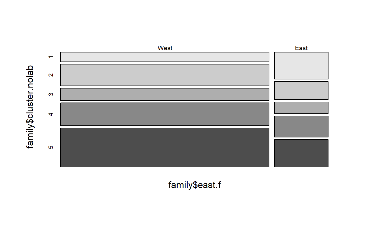
…and print it
row Cell Contents
|-------------------------|
| Count |
| Row Percent |
|-------------------------|
=============================================
family$east.f
family$cluster.nolab West East Total
---------------------------------------------
1 171 124 295
58.0% 42.0% 12.6%
---------------------------------------------
2 386 83 469
82.3% 17.7% 20.0%
---------------------------------------------
3 215 54 269
79.9% 20.1% 11.5%
---------------------------------------------
4 403 96 499
80.8% 19.2% 21.3%
---------------------------------------------
5 688 126 814
84.5% 15.5% 34.7%
---------------------------------------------
Total 1863 483 2346
=============================================We do the same for column percentages, storing the results in an
object named col…
col<-crosstab(family$cluster.nolab,
               family$east.f,
               weight=family$weight40,
               prop.c = TRUE)
… and print it
col Cell Contents
|-------------------------|
| Count |
| Column Percent |
|-------------------------|
=============================================
family$east.f
family$cluster.nolab West East Total
---------------------------------------------
1 171 124 295
9.2% 25.7%
---------------------------------------------
2 386 83 469
20.7% 17.2%
---------------------------------------------
3 215 54 269
11.5% 11.2%
---------------------------------------------
4 403 96 499
21.6% 19.9%
---------------------------------------------
5 688 126 814
36.9% 26.1%
---------------------------------------------
Total 1863 483 2346
79.4% 20.6%
=============================================We can now estimate a multinomial logistic regression model by using
the ?multinom command. Notice that we have to specify the
main dataset (see the data option) and where the weights
are (see the w option). We store the results in an object
named cluster.outcomes…
cluster.outcomes <- multinom(cluster.nolab ~
                              sex.f +
                              east.f +
                              highschool.f,
                              data=family,
                              w=family$weight40)
# weights: 25 (16 variable)
initial value 3776.173113
iter 10 value 3487.915432
iter 20 value 3468.061914
final value 3468.060632
converged…and print its content:
cluster.outcomesCall:
multinom(formula = cluster.nolab ~ sex.f + east.f + highschool.f,
data = family, weights = family$weight40)
Coefficients:
(Intercept) sex.f1 east.fEast highschool.f1
2 0.46803617 0.005987762 -1.127118 0.79893243
3 0.03095799 0.305978164 -1.048926 0.08752612
4 0.64924659 -0.665232375 -1.012543 1.06764454
5 1.08750449 0.230441592 -1.324001 0.46341380
Residual Deviance: 6936.121
AIC: 6968.121 To facilitate the interpretation of the results, we estimate
predicted probabilities for the assignment to each cluster as a function
of being born in East or West Germany by using the ?Effect
command: we have to specify the covariate for which estimating the
predicted probabilities (east.f) and the object where the
regression results are stored (here: cluster.outcomes).
Also in this case, we store the predictions in an object that we name
pred.east:
pred.east <- Effect("east.f", cluster.outcomes)We can print the linear predictions
pred.east
east.f effect (probability) for 1
east.f
      West       East
0.09458644 0.25131721

east.f effect (probability) for 2
east.f
     West      East
0.2090193 0.1799197

east.f effect (probability) for 3
east.f
     West      East
0.1198294 0.1115356

east.f effect (probability) for 4
east.f
     West      East
0.1921056 0.1854349

east.f effect (probability) for 5
east.f
     West      East
0.3844593 0.2717925
One can store the predictions and the upper and lower confidence
intervals values as a data.frame
tidy.pred<-data.frame(pred.east$prob,
                      pred.east$lower.prob,
                      pred.east$upper.prob)
Clusters as predictors
Here we consider satisfaction with family life (a continuous variable
sat1i4 in the family dataset, measured at the end of the observational
window covered by the sequences) as dependent variable in a model where
clusters are the main predictors. We first generate summary statistics
of sat1i4 by cluster by using the ?describeBy command. Note
that we have to specify the group, that is the variable by
which the summary description has to be displayed - here the cluster
variable included in the family dataset. We store the summary in an
object called sat.clu …
sat.clu<-describeBy(family$sat1i4, group=family$cluster)…and print it
sat.clu
 Descriptive statistics by group
group: Early parenthood in cohabitation
   vars   n mean   sd median trimmed  mad min max range  skew
X1    1 292 8.22 1.72      9    8.22 1.48   3  10     7 -1.03
   kurtosis  se
X1     0.53 0.1
----------------------------------------------------
group: LAT and long-lasting cohabitation without children
   vars   n mean   sd median trimmed  mad min max range  skew
X1    1 326 8.08 1.81      8    8.08 1.48   2  10     8 -1.26
   kurtosis  se
X1      1.4 0.1
----------------------------------------------------
group: Early marriage with 1 child
   vars   n mean   sd median trimmed  mad min max range skew kurtosis
X1    1 259 8.21 1.89      9    8.21 1.48   2  10     8 -1.4     1.61
     se
X1 0.12
----------------------------------------------------
group: Long-lasting singleness and childlessness
   vars   n mean   sd median trimmed  mad min max range  skew
X1    1 272 7.54 2.19      8    7.54 1.48   0  10    10 -1.28
   kurtosis   se
X1     1.49 0.13
----------------------------------------------------
group: Early marriage with 2+ children
   vars   n mean   sd median trimmed  mad min max range  skew
X1    1 717 8.37 1.59      9    8.37 1.48   0  10    10 -1.56
   kurtosis   se
X1     3.88 0.06
We can now estimate a linear model for satisfaction with family life
by using the ?lm command. Notice that we have to specify
the main dataset (see the data option) and where the
weights are (see the w option). We store the results in an
object named cluster.predictors…
cluster.predictors <- lm(sat1i4 ~
                           cluster.nolab.f +
                           sex.f +
                           highschool.f +
                           east.f,
                           data=family,
                           w=family$weight40)
…and print the results
cluster.predictors
Call:
lm(formula = sat1i4 ~ cluster.nolab.f + sex.f + highschool.f +
    east.f, data = family, weights = family$weight40)

Coefficients:
     (Intercept)  cluster.nolab.f2  cluster.nolab.f3
         8.33547          -0.34205          -0.16490
cluster.nolab.f4  cluster.nolab.f5            sex.f1
        -0.64746           0.06905          -0.08672
   highschool.f1        east.fEast
        -0.03143           0.01093
To arrange the results nicely, we use the ?tidy command
and store the predictions in an object called
tidy.predictors …
tidy.predictors <- tidy(cluster.predictors)…and print it
tidy.predictors# A tibble: 8 × 5
term estimate std.error statistic p.value
<chr> <dbl> <dbl> <dbl> <dbl>
1 (Intercept) 8.34 0.142 58.8 0
2 cluster.nolab.f2 -0.342 0.159 -2.15 0.0314
3 cluster.nolab.f3 -0.165 0.178 -0.924 0.356
4 cluster.nolab.f4 -0.647 0.158 -4.09 0.0000445
5 cluster.nolab.f5 0.0691 0.146 0.474 0.636
6 sex.f1 -0.0867 0.0879 -0.986 0.324
7 highschool.f1 -0.0314 0.0890 -0.353 0.724
8 east.fEast 0.0109 0.110 0.0995 0.921