Click here to get instructions…
- Please download and unzip the replication files for Chapter 4 ( Chapter04.zip).
- Read
readme.htmland run4-0_ChapterSetup.R. This will create4-0_ChapterSetup.RDatain the sub folderdata/R. This file contains the data required to produce the plots shown below. - You also have to add the function
legend_large_boxto your environment in order to render the tweaked version of the legend described below. You find this file in thesourcefolder of the unzipped Chapter 4 archive. - We also recommend to load the libraries listed in Chapter 4’s
LoadInstallPackages.R
# assuming you are working within .Rproj environment
library(here)

# install (if necessary) and load other required packages
source(here("source", "load_libraries.R"))

# load environment generated in "4-0_ChapterSetup.R"
load(here("data", "R", "4-0_ChapterSetup.RData"))
In chapter 4.2, we apply hierarchical and partitional clustering to family formation sequences. The data come from a sub-sample of the German Family Panel - pairfam. For further information on the study and on how to access the full scientific use file see here.
Hierarchical clustering: Ward’s linkage
We apply a hierarchical cluster analysis by using the command
?hclust to the dissimilarity matrix
partner.child.year.om for the family formation sequences,
computed based on OM with indel=1 and sm=2. We
use non-squared dissimilarities (see the method option) and
weights (see the members option, where we have to specify
to which data.frame the vector with the weights belongs
to).
fam.ward1 <- hclust(as.dist(partner.child.year.om),
                    method = "ward.D",
                    members = family$weight40)
One can combine different heuristics to select the number of
clusters. One is the so-called “elbow” method, based on a line graph
which can be obtained by using the ?fviz_nbclust command.
Notice that we specify here the method option (the method to be used for
estimating the optimal number of clusters) as wss, that is
the total within sum of square. The input of the command is the
dissimilarity matrix partner.child.year.om:
fviz_nbclust(partner.child.year.om,
             FUN = hcut,
             method = "wss",
             barfill = "black",
             barcolor = "black",
             linecolor = "black")
dev.off()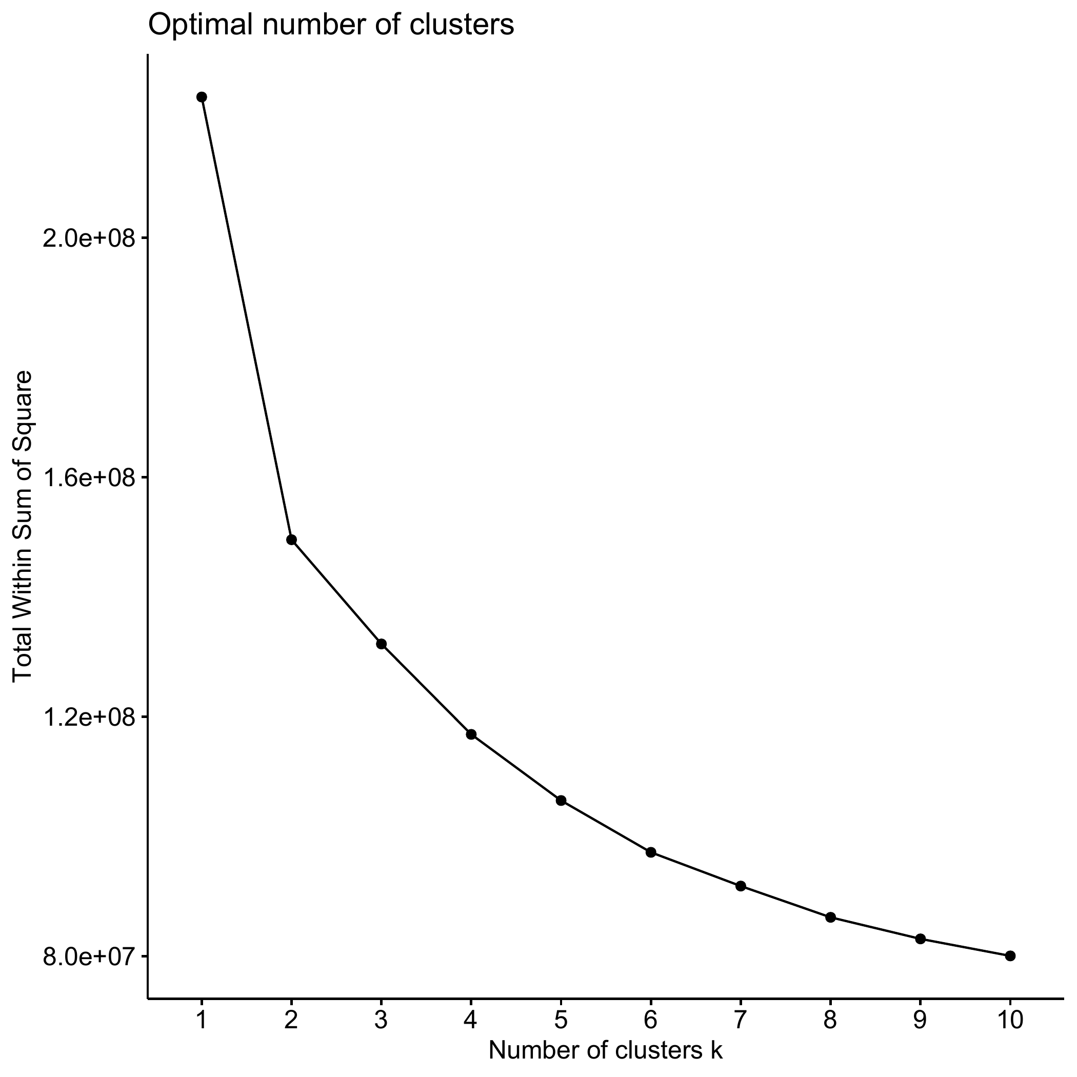
As an alternative or to be used in combination with the elbow method
(please refer Chapter 4.2 in the book), we can use the
?as.clustrange command by using the ?hclust
results (here stored in the object fam.ward1) as input.
?as.clustrange will return a series of cluster quality
indicators. Notice that we have to specify the diss option
by using the dissimilarity matrix of interest and the number of clusters
we want the command to “test” (here 10 in the ncluster
option)
fam.ward.test <- as.clustrange(fam.ward1,
                               diss = partner.child.year.om,
                               weights =family$weight40,
                               ncluster = 10)
Let’s look at the cluster quality indicators
fam.ward.test PBC HG HGSD ASW ASWw CH R2 CHsq R2sq HC
cluster2 0.25 0.30 0.29 0.18 0.18 323.97 0.12 565.24 0.19 0.34
cluster3 0.42 0.51 0.50 0.21 0.21 293.92 0.20 558.60 0.32 0.25
cluster4 0.53 0.69 0.68 0.23 0.23 250.58 0.24 515.74 0.40 0.17
cluster5 0.56 0.74 0.72 0.23 0.23 218.61 0.27 464.61 0.44 0.15
cluster6 0.49 0.69 0.68 0.16 0.17 193.78 0.29 407.00 0.47 0.18
cluster7 0.51 0.72 0.71 0.18 0.18 178.04 0.31 390.32 0.50 0.17
cluster8 0.53 0.77 0.75 0.18 0.18 169.58 0.34 385.53 0.54 0.15
cluster9 0.52 0.81 0.79 0.16 0.17 167.33 0.36 390.71 0.57 0.14
cluster10 0.52 0.83 0.81 0.16 0.17 159.92 0.38 383.55 0.60 0.13We can also visualize the trends in the indicators. Here some selected cluster quality indicators, visualized as z-scores
plot(fam.ward.test, stat = c("ASW", "HG", "PBC", "CH", "R2"),
     lty = 1,
     norm = "zscore",
     main = "CQIs, adjusted by mean and standard deviation (z-scores)",
     lwd = 5,
     ylab="z-scores")

dev.off()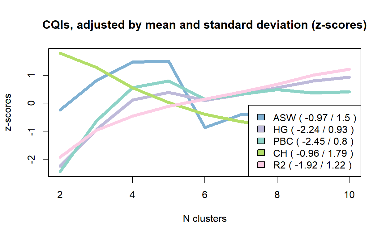
Based on considerations presented in the book, we extract the
5-cluster solution. This can be done with the ?cutree
command, specifying the ?hclust-generate object and the
k number of clusters to be extracted. We store this
information into an object called fam.ward.5cl
fam.ward.5cl <-cutree(fam.ward1, k = 5)…that we add to the main data.frame
family:
family$fam.ward.5cl<-fam.ward.5clBecause we want to illustrate how to compare different cluster solutions, we also extract 4 clusters and repeat the procedure
fam.ward.4cl <-cutree(fam.ward1, k = 4)

family$fam.ward.4cl<-fam.ward.4cl
We can now cross-tabulate the 4- and 5-cluster solutions storing the table into an object…
comp.ward<-table(fam.ward.5cl, fam.ward.4cl)… that we can print at our convenience:
comp.ward fam.ward.4cl
fam.ward.5cl 1 2 3 4
1 289 0 0 0
2 0 353 0 0
3 0 147 0 0
4 0 0 386 0
5 0 0 0 691Partitional clustering: PAM
We use the ?wcKMedRange command to obtain the cluster
quality indicators for a number of clusters between 2 and 10 (see the
kvals option) using the PAM algorithm. We also specify
weights (see weights option). Further, we specify the
initialclust option by using the
?hclust-generated object we used above
fam.pam.ward <- wcKMedRange(partner.child.year.om,
                            weights = family$weight40,
                            kvals = 2:10,
                            initialclust = fam.ward1)
Let’s consider the cluster quality criteria for this PAM clustering
fam.pam.ward PBC HG HGSD ASW ASWw CH R2 CHsq R2sq HC
cluster2 0.43 0.52 0.50 0.22 0.23 348.56 0.13 676.34 0.22 0.24
cluster3 0.49 0.61 0.60 0.24 0.24 318.83 0.21 642.69 0.35 0.20
cluster4 0.56 0.72 0.71 0.25 0.25 272.71 0.26 577.80 0.43 0.15
cluster5 0.57 0.77 0.76 0.25 0.25 237.22 0.29 521.18 0.47 0.13
cluster6 0.48 0.71 0.69 0.19 0.19 212.05 0.31 462.26 0.50 0.18
cluster7 0.49 0.75 0.73 0.20 0.20 200.27 0.34 450.94 0.54 0.16
cluster8 0.50 0.78 0.77 0.21 0.21 194.91 0.37 456.15 0.58 0.15
cluster9 0.50 0.81 0.79 0.20 0.20 187.59 0.39 448.61 0.61 0.14
cluster10 0.52 0.87 0.85 0.23 0.24 184.81 0.42 471.62 0.64 0.11We first extract a 4-cluster solution
fam.pam.ward.4cl<-fam.pam.ward$clustering$cluster4… attach the vector with the 4-cluster solution to the main
data.frame:
family$fam.pam.ward.4cl<-fam.pam.ward.4cl… and re-label clusters from 1 to 4 instead of medoid identifier by
using the ?recode command:
family$fam.pam.ward.4cl<-car::recode(family$fam.pam.ward.4cl,
                                     "1532=1; 1664=2; 1643=3; 985=4")
We then extract the 5-cluster solution with the same procedure:
fam.pam.ward.5cl<-fam.pam.ward$clustering$cluster5

family$fam.pam.ward.5cl<-fam.pam.ward.5cl

family$fam.pam.ward.5cl<-car::recode(family$fam.pam.ward.5cl,
                                     "982=1; 790=2; 373=3; 1643=4; 985=5")
We want to compare the 4 and 5-cluster solutions for PAM+Ward
clustering. We can use the ?table command and store the
table into an object…
comp.pam.ward<-table(family$fam.pam.ward.5cl, family$fam.pam.ward.4cl)…to be printed at our convenience
comp.pam.ward
      1   2   3   4
  1 235  12   2  43
  2  54 240  11  21
  3   7 232  14   6
  4   2   4 266   0
  5   0  23   0 694
We now compute the average silhouette width by cluster: we can use
the ?silhouette command and specify the dissimilarity
matrix in the dmatrix option. We do that for the 4- and the
5-cluster solutions. As usual, we store the results into an object…
silh.pam.ward.5cl <- silhouette(family$fam.pam.ward.5cl,
                                dmatrix = partner.child.year.om)
silh.pam.ward.4cl <- silhouette(family$fam.pam.ward.4cl,
                                dmatrix = partner.child.year.om)
…that can be plotted:
par(mfrow=c(1,2))
plot(silh.pam.ward.4cl, main = "(a) four-cluster solution",
     col="grey", border=NA)
plot(silh.pam.ward.5cl, main = "(b) five-cluster solution",
     col="grey", border=NA)

dev.off()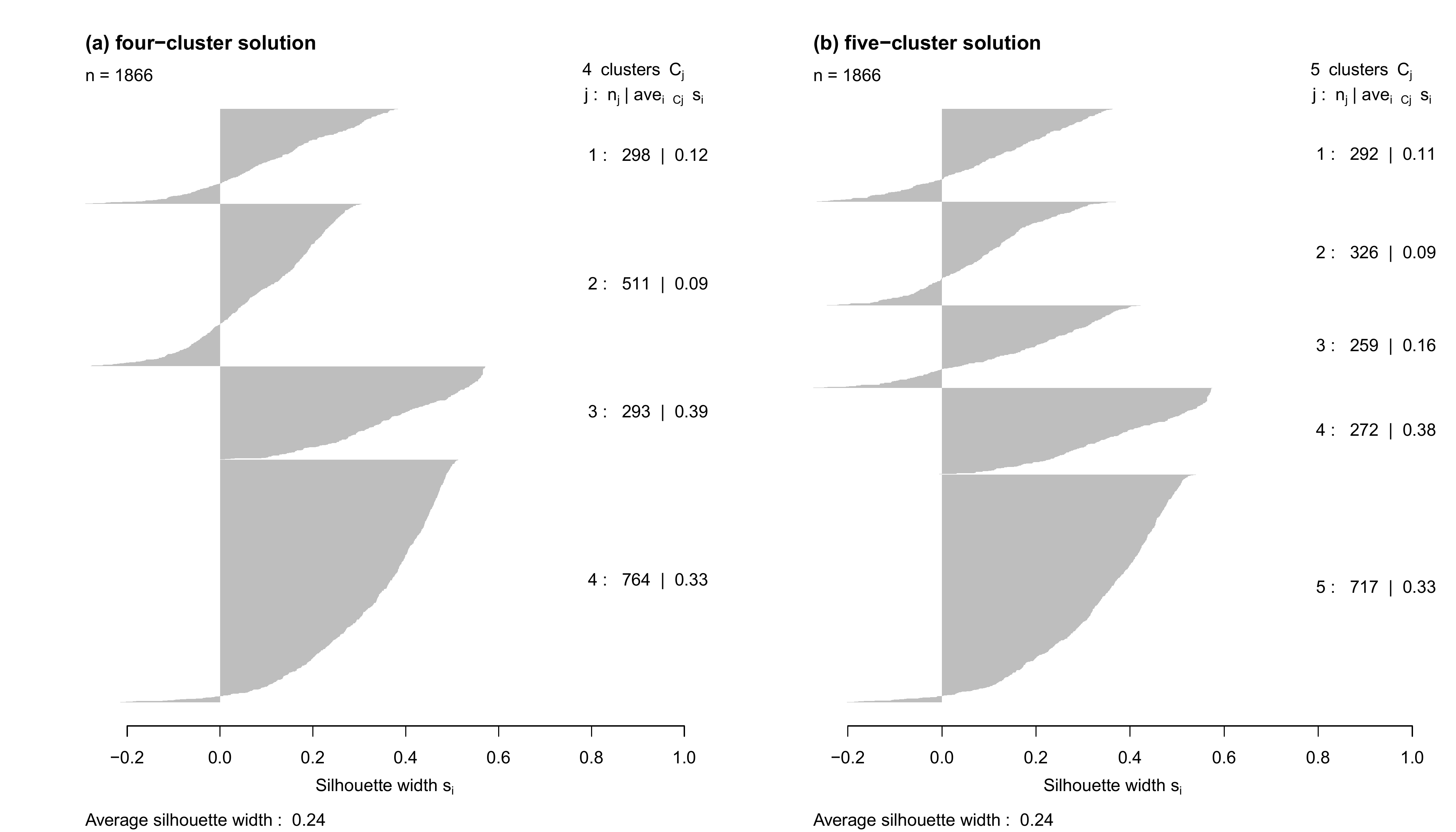
We now proceed with the 5-cluster solution and generate substantively meaningful label for the clusters. Notice that to do this, we need to first visualize the clusters and ideally explore each of them with the descriptive tools presented in Chapter 2
fam.pam.ward.lab.5cl <- c("Early parenthood in cohabitation",
                          "LAT and long-lasting cohabitation without children",
                          "Early marriage with 1 child",
                          "Long-lasting singleness and childlessness",
                          "Early marriage with 2+ children")
We attach the labels to the clusters by generating a factor variable:
beware of the order of the clusters (option levels) and of
the labels (option labels which is specified with the
object created above), as it has to correspond!
fam.pam.ward.factor.5cl <- factor(family$fam.pam.ward.5cl,
                                  levels = c(1,2,3,4,5),
                                  labels=fam.pam.ward.lab.5cl)
We can now attach the cluster-vector (with labels) to the main
data.frame:
family$fam.pam.ward.factor.5cl<-fam.pam.ward.factor.5clTo be sure, one might want to confirm that family with the newly attached vectors is a whole data frame
family<-data.frame(family)Among the many options for visualization introduced in Chapter 2, we
use the relative frequency plot. The standard ?seqplot.rf
command for this graph produces a combined figure: the sequences and the
distance-to-medoid plot. One can also plot only one of the two by
specifying the option which.plot. In the archive
Chapter04.zip in the download area of this webpage, you can find a code
to efficiently plot only the sequences part of the relative frequency
plot especially if you want to plot the clusters in the same figure.
Assuming you are working within .Rproj environment, you can
use the following code
source(here("source", "rfplotsleft.R"))Notice that we recommend to always display the distance-to-medoid
plot for each cluster at least in the appendix of your article: an
example of this can be found in Struffolino and Van Winkle 2021
(open-access version here).
For a nice display of the clusters using the sourced code
rfplotsleft.R, we first generate separate objects
containing the sequences allocated to each clusters:
cl1_5cl<-(partner.child.year.seq[family$fam.pam.ward.factor.5cl=="Early parenthood in cohabitation",1:22])

cl2_5cl<-(partner.child.year.seq[family$fam.pam.ward.factor.5cl=="LAT and long-lasting cohabitation without children",1:22])

cl3_5cl<-(partner.child.year.seq[family$fam.pam.ward.factor.5cl=="Early marriage with 1 child",1:22])

cl4_5cl<-(partner.child.year.seq[family$fam.pam.ward.factor.5cl=="Long-lasting singleness and childlessness",1:22])

cl5_5cl<-(partner.child.year.seq[family$fam.pam.ward.factor.5cl=="Early marriage with 2+ children",1:22])
We then compute the dissimilarity matrix for each separate cluster:
cl1_5cl.om<- seqdist(cl1_5cl, method="OM", indel=1, sm= "CONSTANT")

cl2_5cl.om<- seqdist(cl2_5cl, method="OM", indel=1, sm= "CONSTANT")

cl3_5cl.om<- seqdist(cl3_5cl, method="OM", indel=1, sm= "CONSTANT")

cl4_5cl.om<- seqdist(cl4_5cl, method="OM", indel=1, sm= "CONSTANT")

cl5_5cl.om<- seqdist(cl5_5cl, method="OM", indel=1, sm= "CONSTANT")
In preparation for the graph, we generate labels for x-axis, 22 time-points in steps of 2, labeled with numbers from 18 to 40, that is the age span our sequences cover
count <- seq(from = 0, to = 22, by = 2)
years <- seq(from = 18, to = 40, by = 2)
We now code the combined relative frequency plot (only the sequences
part) to display all clusters at once: for each cluster, we set 50
medoid sequences. Notice that here we use the seqplot.rf.l
command that is included in the sourced code rfplotsleft.R.
Note that the line below the x-axis label “Age” of each cluster plot
reports the R2 and F-stat values generated by running the standard
?seqplot.rf command. It is your choice to report them, but
we recommend to do so. Unfortunately, for now our solution is to impute
this information manually as you can see in the code below:
def.par <- par(no.readonly = TRUE)

par(oma = c(0, 2, 2, 0))

m <- matrix(c(1,2,3,4,5,6), 3, 2, byrow = TRUE)
nf <- layout(mat = m, heights = c(0.8,0.8,0.8))
layout.show(nf)

par(mar = c(5, 3, 3, 3))

seqplot.rf.l(cl1_5cl, diss=cl1_5cl.om,
             k=50, xlab="",cex.main=1.6,
             title="1.Early parenthood in cohabitation (15.7%)",
             ylab=FALSE,
             cex.lab=1.4, axes=FALSE)
mtext("Age",side = 1, line = 2.5, cex=0.9)
mtext("Medoid sequences",side = 2, line = 1.5, cex=0.9)
mtext("R2=0.27 / F-stat=1.79",side = 1, line = 4, cex=0.7)
axis(1, at = count, labels = years, font = 1, cex.axis = 1, lwd = 1)

seqplot.rf.l(cl2_5cl, diss=cl2_5cl.om,
             k=50, xlab="",cex.main=1.6,
             title="2.LAT/long-lasting cohabitation without children (17.5%)",
             ylab=FALSE,
             cex.lab=1.4, axes=FALSE)
mtext("Age",side = 1, line = 2.5, cex=0.9)
mtext("Medoid sequences",side = 2, line = 1.5, cex=0.9)
mtext("R2=0.30 / F-stat=2.40",side = 1, line = 4, cex=0.7)
axis(1, at = count, labels = years, font = 1, cex.axis = 1, lwd = 1)

seqplot.rf.l(cl3_5cl, diss=cl3_5cl.om,
             k=50, xlab="",cex.main=1.6,
             title="3.Early marriage with 1 child (13.9%)",
             ylab=FALSE,
             cex.lab=1.4, axes=FALSE)
mtext("Age",side = 1, line = 2.5, cex=0.9)
mtext("Medoid sequences",side = 2, line = 1.5, cex=0.9)
mtext("R2=0.45 / F-stat=3.47",side = 1, line = 4, cex=0.7)
axis(1, at = count, labels = years, font = 1, cex.axis = 1, lwd = 1)

seqplot.rf.l(cl4_5cl, diss=cl4_5cl.om,
             k=50, xlab="",cex.main=1.6,
             title="4.Long-lasting singleness and childlessness (14.6%)",
             ylab=FALSE,
             cex.lab=1.4, axes=FALSE)
mtext("Age",side = 1, line = 2.5, cex=0.9)
mtext("Medoid sequences",side = 2, line = 1.5, cex=0.9)
mtext("R2=0.32 / F-stat=2.13",side = 1, line = 4, cex=0.7)
axis(1, at = count, labels = years, font = 1, cex.axis = 1, lwd = 1)

seqplot.rf.l(cl5_5cl, diss=cl5_5cl.om,
             k=50, xlab="",cex.main=1.6,
             title="5.Early marriage with 2+ children (38.4%)",
             ylab=FALSE,
             cex.lab=1.4, axes=FALSE)
mtext("Age",side = 1, line = 2.5, cex=0.9)
mtext("Medoid sequences",side = 2, line = 1.5, cex=0.9)
mtext("R2=0.35 / F-stat=7.26",side = 1, line = 4, cex=0.7)
axis(1, at = count, labels = years, font = 1, cex.axis = 1, lwd = 1)

plot(1, type = "n", axes=FALSE, xlab="", ylab="")
legend(x = "center",inset = 0,
       legend = longlab.partner.child,
       col=colspace.partner.child,
       lwd=10, cex=1.3, ncol=1)

dev.off()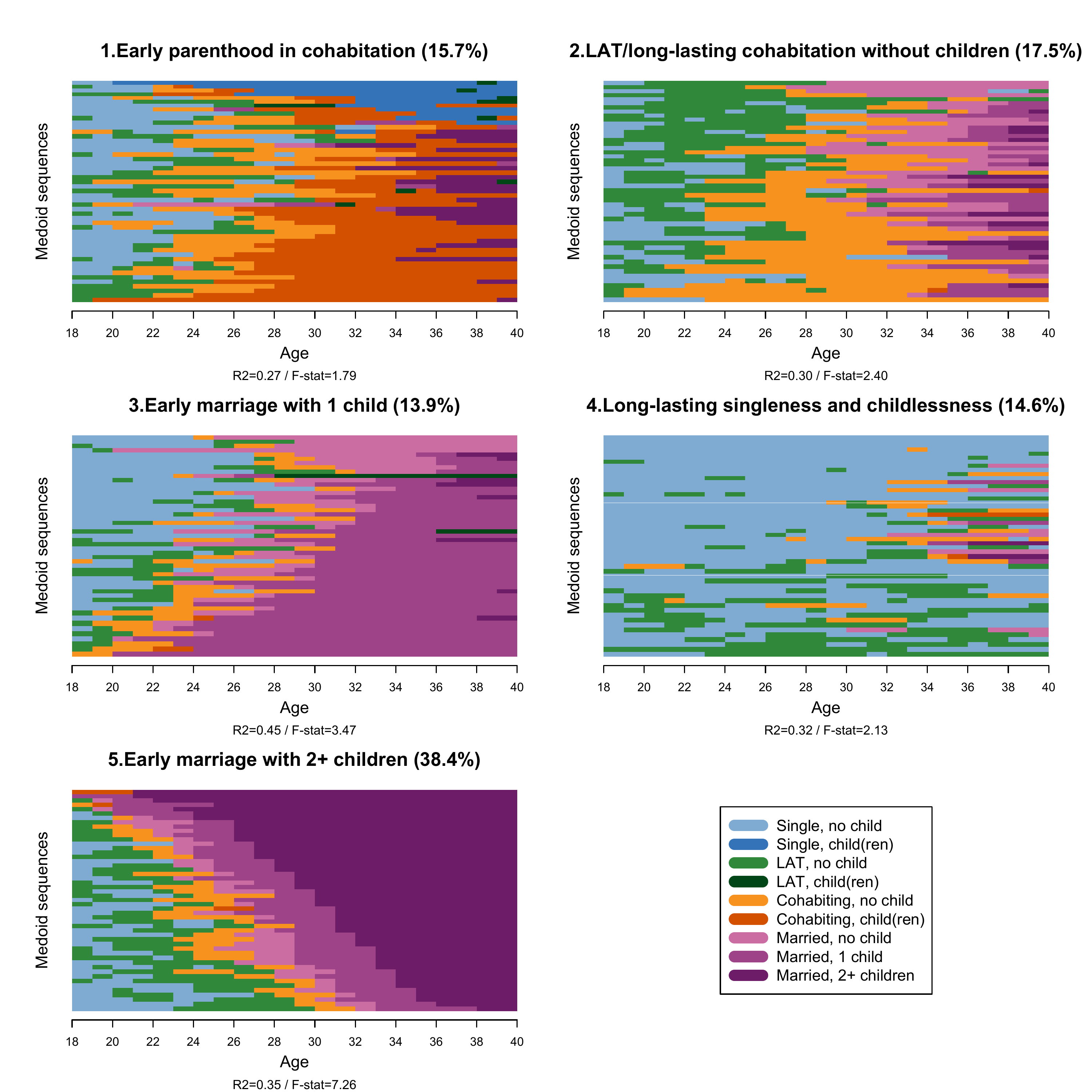
Visualizing clustering options with MDS
We use the ?cmdscale to calculate the multidimensional
scaling of the dissimilarity matrix partner.child.year.om.
We the k option (the maximum dimension of the space which
the data are to be represented in) at 2
mds.year.om<-cmdscale(partner.child.year.om, k = 2)For illustrative purposes, we extract 3 clusters based on the hierarchical clustering (Ward) and the PAM clustering following the procedure presented in detail above
# Ward
mds_ward <- hclust(as.dist(partner.child.year.om),
                   method = "ward.D",
                   members = family$weight40)

# Cut the clustering at 3
mds_ward_3 <-cutree(mds_ward, k = 3)

#PAM
mds_pam <- wcKMedoids(partner.child.year.om, k = 3)

# Extract the 3 clusters
mds_pam <- mds_pam$clustering

# Re-label the clusters 1 to 3 instead of medois id
mds_pam <- car::recode(mds_pam, "156=1; 985=2; 1735=3")
We can now use the objects mds.year.om,
mds_ward, mds_pam to visualize the
distribution of the sequences in the samples by cluster (extracted by
using two different clustering method) in a bi-dimensional space
par(mfrow=c(1,2))

par(mar = c(7, 7, 3, 3))

plot(mds.year.om, type = "n",
     main="Hierachical clustering (Ward's linkage)",
     ylab="Coordinate 2",
     xlab="Coordinate 1",
     cex.lab=1.7,
     cex.main=1.7)
points(mds.year.om[mds_ward_3 == 1, ], pch = 19, col = "black")
points(mds.year.om[mds_ward_3 == 2, ], pch = 21, col = "black")
points(mds.year.om[mds_ward_3 == 3, ], pch = 24, col = "black")

legend("bottomright", pch = c(19,21,24), legend = c("cluster 1", "cluster 2", "cluster 3"), cex=1.6)
plot(silh.pam.ward.5cl, main = "(b) MDS PAM", col="grey", border=NA)

par(mar = c(7, 7, 3, 3))

plot(mds.year.om, type = "n",
     main="Partitional clustering (k-medoid)",
     ylab="Coordinate 2",
     xlab="Coordinate 1",
     cex.lab=1.7,
     cex.main=1.7)
points(mds.year.om[mds_pam == 1, ], pch = 19, col = "black")
points(mds.year.om[mds_pam == 2, ], pch = 21, col = "black")
points(mds.year.om[mds_pam == 3, ], pch = 24, col = "black")

legend("bottomright", pch = c(19,21,24), legend = c("cluster 1", "cluster 2", "cluster 3"), cex=1.6)

dev.off()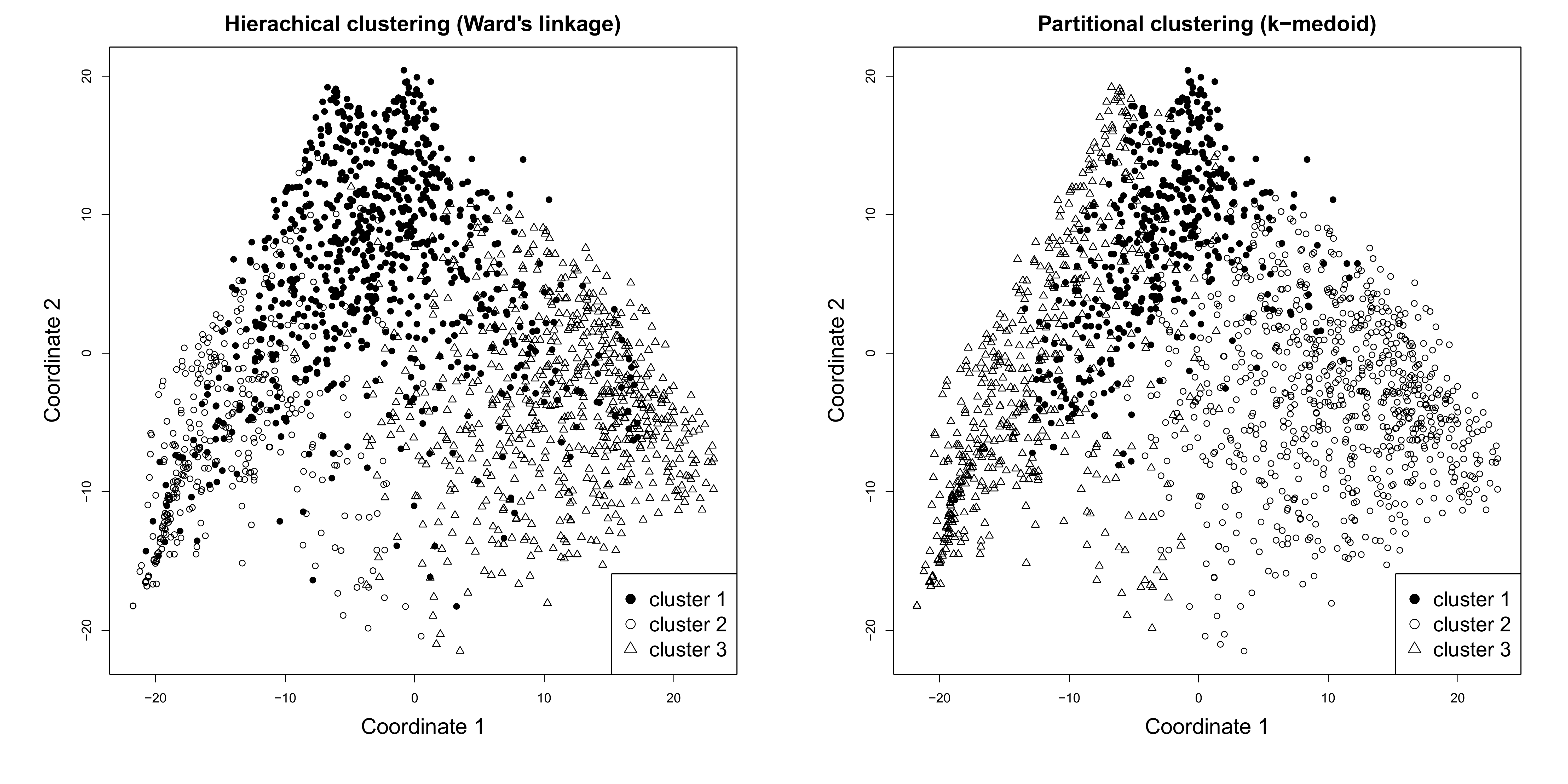
Comparison between different time granularities
We adopt the same strategy used above for yearly sequences to the case of monthly sequences.
Hierarchical cluster analysis, non-squared dissimilarities, weighted
fam.ward1.month <- hclust(as.dist(partner.child.month.om),
                          method = "ward.D",
                          members = family$weight40)
PAM cluster analysis initialized with Ward, weighted
fam.pam.ward.month <- wcKMedRange(partner.child.month.om,
                                  weights = family$weight40,
                                  kvals = 2:10,
                                  initialclust = fam.ward1.month)
Print the quality test for different cluster solutions
fam.pam.ward.month PBC HG HGSD ASW ASWw CH R2 CHsq R2sq HC
cluster2 0.41 0.47 0.47 0.22 0.22 336.85 0.13 645.83 0.22 0.25
cluster3 0.51 0.61 0.60 0.23 0.24 304.42 0.21 613.04 0.34 0.19
cluster4 0.49 0.62 0.62 0.21 0.21 265.61 0.25 548.78 0.41 0.20
cluster5 0.51 0.68 0.68 0.21 0.21 234.84 0.29 495.70 0.46 0.17
cluster6 0.51 0.72 0.72 0.21 0.21 219.85 0.32 487.01 0.51 0.16
cluster7 0.52 0.76 0.76 0.22 0.22 208.00 0.35 473.79 0.55 0.14
cluster8 0.50 0.76 0.76 0.20 0.20 195.64 0.37 450.95 0.57 0.15
cluster9 0.51 0.80 0.80 0.22 0.23 190.03 0.39 458.18 0.61 0.13
cluster10 0.53 0.85 0.85 0.24 0.24 185.71 0.42 474.29 0.65 0.10Extract the 5-cluster solution
fam.pam.ward.month.5cl<-fam.pam.ward.month$clustering$cluster5Attach the vector with the 5-cluster solution to the main
data.frame
family$fam.pam.ward.month.5cl<-fam.pam.ward.month.5clRe-label clusters from 1 to 5 instead of medoid identifiers
family$fam.pam.ward.month.5cl<-car::recode(family$fam.pam.ward.month.5cl,
                                           "1652=1; 1032=2; 412=3; 869=4; 927=5")
We can now compare the cluster assignment in the case of yearly and monthly data. In both cases we extracted 5 clusters from the PAM+Ward option…
comp.y.m<-table(family$fam.pam.ward.5cl, family$fam.pam.ward.month.5cl)…and print the resulting table
comp.y.m
      1   2   3   4   5
  1 222  38   7   3  22
  2  91 108 115  11   1
  3   0  35 212  11   1
  4   5  29   2 236   0
  5   2 217   5   0 493