Click here to get instructions…
- Please download and unzip the replication files for Chapter 3 ( Chapter03.zip).
- Read
readme.htmland run3-0_ChapterSetup.R. This will create3-0_ChapterSetup.RDatain the sub folderdata/R. This file contains the data required to produce the plots shown below. - You also have to add the function
legend_large_boxto your environment in order to render the tweaked version of the legend described below. You find this file in thesourcefolder of the unzipped Chapter 3 archive. - We also recommend to load the libraries listed in Chapter 3’s
LoadInstallPackages.R
# assuming you are working within .Rproj environment
library(here)

# install (if necessary) and load other required packages
source(here("source", "LoadInstallPackages.R"))

# load environment generated in "3-0_ChapterSetup.R"
load(here("data", "R", "3-0_ChapterSetup.RData"))
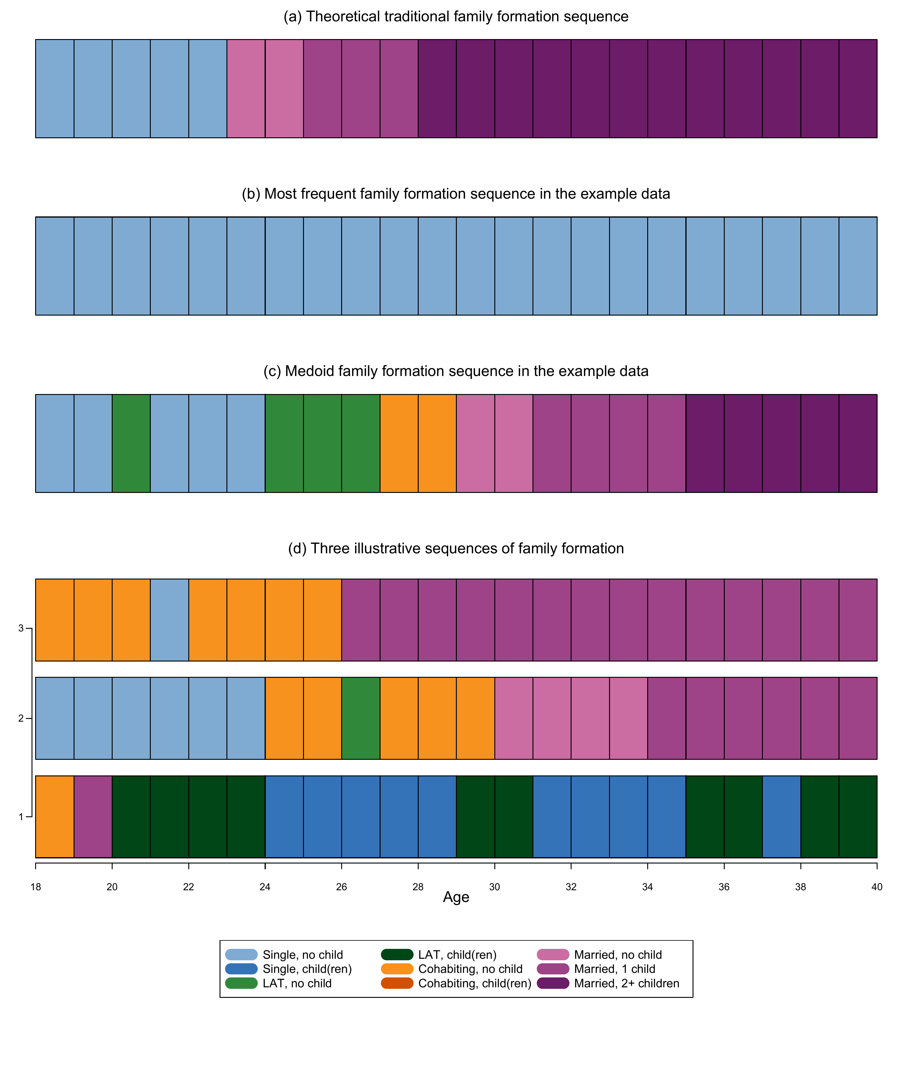
In chapter 3.7, we introduce techniques to compare all sequences in a dataset to a reference sequences instead of conducting a full-sample pairwise comparison. The data come from a sub-sample of the German Family Panel - pairfam. For further information on the study and on how to access the full scientific use file see here.
Defining a theoretical sequence
First, we generate an object that contains the theoretical sequence id the SPS format of the same length of the sequences in the sample:
theo.seq<-as.matrix("(S,5)-(MAR,2)-(MARc1,3)-(MARc2+,12)")…and print it
theo.seq [,1]
[1,] "(S,5)-(MAR,2)-(MARc1,3)-(MARc2+,12)"We then recode the theoretical sequence from SPS to STS and overwrite the object that contains it
theo.seq <- seqformat(theo.seq, from = "SPS", to = "STS")We overwrite it again, by formally define it as a sequence using the
TraMineR ?seqdef command:
theo.seq<-seqdef(theo.seq,
                 states = shortlab.partner.child,
                 alphabet = shortlab.partner.child,
                 xtstep = 1)
We can now compute the dissimilarity between the theoretical sequence
and all sequences in the data. Here we use OM with constant substitution
costs and indel =1. The theo.seq object has to
be specified as argument to the option refseq
dist.theo<-seqdist(partner.child.year.seq,
                   method = "OM",
                   indel = 1,
                   sm = "CONSTANT",
                   refseq = theo.seq)
Identify the most frequent sequence in the data
We can identify the most frequent sequence by using the
?seqtab command and specify the idxs as
follows and store it in a separate object, here called
mostfreq.seq
mostfreq.seq<-seqtab(partner.child.year.seq,
                     idxs = 1,
                     weighted = FALSE,
                     format = "SPS")
We print the most frequent sequence
mostfreq.seq Freq Percent
S/22 14 0.75… and compute the dissimilarity between the most frequent sequence
and all sequences in the data. The mostfreq.seq object has
to be specified as argument to the option refseq
dist.mostfreq<-seqdist(partner.child.year.seq,
                       method = "OM",
                       indel = 1,
                       sm = "CONSTANT",
                       refseq = mostfreq.seq)
Identify the medoid sequence in the data
First, we have to compute a dissimilarity matrix, here we use OM with
constant substitution costs of 2 and indel=1
om.s2.i1<-seqdist(partner.child.year.seq,
                  method = "OM",
                  indel = 1,
                  sm = "CONSTANT")
We can then identify the medoid by using the ?disscenter
command and specify the medoids.index options as
follows
medoid.seq <- disscenter(om.s2.i1,
                         medoids.index="first")
The medoid can be also printed directly by using the following code
print(partner.child.year.seq[medoid.seq,],
      format="SPS")
Sequence
1544 (S,2)-(LAT,1)-(S,3)-(LAT,3)-(COH,2)-(MAR,2)-(MARc1,4)-(MARc2+,5)We can now compute the dissimilarity between the medoid sequence and
all sequences in the data. The medoid.seq object has to be
specified as argument to the option refseq
dist.medoid<-seqdist(partner.child.year.seq,
                     method = "OM",
                     indel = 1,
                     sm = "CONSTANT",
                     refseq = medoid.seq[1])
Summary and visual comparison
We display the dissimilarity values for the first three sequences in the sample and the three reference sequences:
dist.theo[1:3] 1 2 3
42 24 36 dist.mostfreq[1:3] 1 2 3
44 32 42 dist.medoid[1:3] 1 2 3
40 16 30 For a visual comparison, here is the version in colors of Figure 3.3, displayed in black and white in the book:
Here the code to generate the figure above
layout.fig1 <- layout(matrix(c(1,2,3,4,5), 5, 1, byrow = TRUE),
                      heights = c(.20,.20,.20,.42,.20))
layout.show(layout.fig1)

par(mar=c(3, 3, 3, 2))

#theoretical
seqiplot(theo.seq,
         with.legend=FALSE,
         border = TRUE,
         axes = FALSE,
         yaxis = FALSE, ylab = NA,
         main="",
         cex.main = 2,
         cpal = colspace.partner.child)
mtext(text = "(a) Theoretical traditional family formation sequence",
      side = 3,#side 1 = bottom
      line = 1,
      las=1)

#most freqent
seqiplot(mostfreq.seq,
         with.legend=FALSE,
         border = TRUE,
         axes = FALSE,
         yaxis = FALSE, ylab = NA,
         main="",
         cex.main = 2,
         cpal = colspace.partner.child)
mtext(text = "(b) Most frequent family formation sequence in the example data",
      side = 3,#side 1 = bottom
      line = 1,
      las=1)

# medoid
seqiplot(partner.child.year.seq[medoid.seq,],
         with.legend=FALSE,
         border = TRUE,
         axes = FALSE,
         yaxis = FALSE, ylab = NA,
         main="",
         cex.main = 2,
         cpal = colspace.partner.child)
mtext(text = "(c) Medoid family formation sequence in the example data",
      side = 3,#side 1 = bottom
      line = 1,
      las=1)

#example 3 seq
seqiplot(partner.child.year.seq [1:3, ],
         with.legend=FALSE,
         border = TRUE,
         axes = FALSE,
         yaxis = FALSE, ylab = NA,
         main="",
         cex.main = 2,
         cpal = colspace.partner.child,
         weighted=FALSE)

par(mgp=c(3,1,-0.5)) # adjust parameters for x-axis
axis(1, at=(seq(0,22, 2)), labels = seq(18,40, by = 2))
par(mgp=c(3,1,0.3), las=1)
axis(2, at=c(0.7,1.9,3), labels = c(1,2,3))
mtext(text = "(d) Three illustrative sequences of family formation",
      side = 3,#side 1 = bottom
      line = 1)
mtext(text = "Age",
      side = 1,#side 1 = bottom
      line = 2)

#legend
plot(NULL ,xaxt='n',yaxt='n',bty='n',ylab='',xlab='', xlim=0:1, ylim=0:1)

legend(x = "top",inset = 0,
       legend = longlab.partner.child,
       col=colspace.partner.child,
       lwd=12,
       cex=1.2,
       ncol=3,lty = 7)

par(mar=c(1, 1, 4, 1))

title(main = "",
      line = 2, font.main = 1)

dev.off()