Sequence Analysis - Companion Site: Correlation for dissimilarity matrices

Click here to get instructions…

Please download and unzip the replication files for Chapter 3 ( Chapter03.zip).
Read readme.html and run 3-0_ChapterSetup.R. This will create 3-0_ChapterSetup.RData in the sub folder data/R. This file contains the data required to produce the plots shown below.
You also have to add the function legend_large_box to your environment in order to render the tweaked version of the legend described below. You find this file in the source folder of the unzipped Chapter 3 archive.
We also recommend to load the libraries listed in Chapter 3’s LoadInstallPackages.R

# assuming you are working within .Rproj environment
library(here)

# install (if necessary) and load other required packages
source(here("source", "load_libraries.R"))

# load environment generated in "3-0_ChapterSetup.R"
load(here("data", "R", "3-0_ChapterSetup.RData"))

In chapter 3.5, we consider how to compute a correlation matrix of sequences’ pairwise dissimilarity matrices obtained using different strategies. The data come from a sub-sample of the German Family Panel - pairfam. For further information on the study and on how to access the full scientific use file see here.

Preparatory work: computing the dissimilarity matrices to be compared

Two OM-based with different substitution costs, first equal to 2 and then equal to 1:

costs.sm2 <- matrix(
  c(0,2,2,2,2,2,2,2,2,
    2,0,2,2,2,2,2,2,2,
    2,2,0,2,2,2,2,2,2,
    2,2,2,0,2,2,2,2,2,
    2,2,2,2,0,2,2,2,2,
    2,2,2,2,2,0,2,2,2,
    2,2,2,2,2,2,0,2,2,
    2,2,2,2,2,2,2,0,2,
    2,2,2,2,2,2,2,2,0
  ),
  nrow = 9, 
  ncol = 9, 
  byrow = TRUE)

costs.sm1 <- matrix(
  c(0,1,1,1,1,1,1,1,1,
    1,0,1,1,1,1,1,1,1,
    1,1,0,1,1,1,1,1,1,
    1,1,1,0,1,1,1,1,1,
    1,1,1,1,0,1,1,1,1,
    1,1,1,1,1,0,1,1,1,
    1,1,1,1,1,1,0,1,1,
    1,1,1,1,1,1,1,0,1,
    1,1,1,1,1,1,1,1,0
  ),
  nrow = 9, 
  ncol = 9, 
  byrow = TRUE)

OM with substitution costs based on state properties (or features):

partner <- c(0, 0, 1, 1, 1, 1, 1,1,1)
child <- c(0,1,0,1,0,1,0,1,2)

alphabetprop <- data.frame(partner = partner, 
                           child = child)

rownames(alphabetprop) <- alphabet(partner.child.year.seq)

prop <- seqcost(partner.child.year.seq, 
                method="FEATURES",
                state.features = alphabetprop)

OM with theory-based substitution costs:

theo <- matrix(
  c(0,1,2,2,2,2,2,2,2,
    1,0,2,2,2,2,2,2,2,
    2,2,0,1,2,2,2,2,2,
    2,2,1,0,2,2,2,2,2,
    2,2,2,2,0,1,2,2,2,
    2,2,2,2,1,0,2,2,2,
    2,2,2,2,2,2,0,1,1,
    2,2,2,2,2,2,1,0,1,
    2,2,2,2,2,2,1,1,0),
  nrow = 9, 
  ncol = 9, 
  byrow = TRUE,
  dimnames = list(shortlab.partner.child, 
                  shortlab.partner.child))

Correlation between the different dissimilarity matrices

We now compute the dissimilarity matrices with different options to be compared:

om.s2.i1<-seqdist(partner.child.year.seq, 
                  method = "OM", 
                  indel = 1,
                  sm = costs.sm2)

om.s1.i4<-o<-seqdist(partner.child.year.seq, 
                     method = "OM", 
                     indel = 2,
                     sm = costs.sm1)

om.prop<-seqdist(partner.child.year.seq, 
                 method = "OM", 
                 indel = 1,
                 sm = prop$sm)

om.theo<-seqdist(partner.child.year.seq, 
                 method = "OM", 
                 indel = 1,
                 sm = theo)

trate<-seqdist(partner.child.year.seq, 
               method = "OM", 
               indel=1, 
               sm= "TRATE")
lcs<-seqdist(partner.child.year.seq, 
             method = "LCS")

ham<-seqdist(partner.child.year.seq, 
             method = "HAM")

dhd<-seqdist(partner.child.year.seq, 
             method = "DHD")

Further, we have to create a data.frame that bring together the various dissimilarity matrices:

diss.partner.child <- data.frame(
  OMi1s2 = vech(om.s2.i1),
  OMi2s1 = vech(om.s1.i4),
  prop = vech(om.prop),
  theo = vech(om.theo),
  trate = vech(trate),
  lcs = vech(lcs),
  ham = vech(ham),
  dhd = vech(dhd)
)

We can now calculate the correlation between the various dissimilarity matrices:

corr.partner.child <- cor(diss.partner.child)

…and display the resulting correlation matrix

corr.partner.child

          OMi1s2    OMi2s1      prop      theo     trate       lcs
OMi1s2 1.0000000 0.8555472 0.6357089 0.9266681 0.9970669 1.0000000
OMi2s1 0.8555472 1.0000000 0.6473117 0.8148489 0.8613480 0.8555472
prop   0.6357089 0.6473117 1.0000000 0.6760080 0.6606818 0.6357089
theo   0.9266681 0.8148489 0.6760080 1.0000000 0.9340574 0.9266681
trate  0.9970669 0.8613480 0.6606818 0.9340574 1.0000000 0.9970669
lcs    1.0000000 0.8555472 0.6357089 0.9266681 0.9970669 1.0000000
ham    0.8548552 0.9998744 0.6470960 0.8141966 0.8606506 0.8548552
dhd    0.8658035 0.9953723 0.6769755 0.8311569 0.8769376 0.8658035
             ham       dhd
OMi1s2 0.8548552 0.8658035
OMi2s1 0.9998744 0.9953723
prop   0.6470960 0.6769755
theo   0.8141966 0.8311569
trate  0.8606506 0.8769376
lcs    0.8548552 0.8658035
ham    1.0000000 0.9953943
dhd    0.9953943 1.0000000

Correlation between the different normalized dissimilarity matrices

It is wise to compute the dissimilarity matrices with different options to be compared by setting the normalization method (see ?seqdist to learn more about this):

om.s2.i1.n<-seqdist(partner.child.year.seq, 
                    method = "OM", 
                    indel = 1,
                    sm = costs.sm2, 
                    norm="auto")

om.s1.i4.n<-o<-seqdist(partner.child.year.seq, 
                       method = "OM", 
                       indel = 2,
                       sm = costs.sm1, 
                       norm="auto")

om.prop.n<-seqdist(partner.child.year.seq, 
                   method = "OM", 
                   indel = 1,
                   sm = prop$sm, 
                   norm="auto")

om.theo.n<-seqdist(partner.child.year.seq,
                   method = "OM", 
                   indel = 1,
                   sm = theo, 
                   norm="auto")

trate.n<-seqdist(partner.child.year.seq,
                 method = "OM", 
                 indel=1, 
                 sm= "TRATE", 
                 norm="auto")

lcs.n<-seqdist(partner.child.year.seq,
               method = "LCS", 
               norm="auto")

ham.n<-seqdist(partner.child.year.seq, 
               method = "HAM", 
               norm="auto")

dhd.n<-seqdist(partner.child.year.seq, 
               method = "DHD", 
               norm="auto")

Also in this case, we create a data.frame of the various normalized dissimilarity matrices:

diss.partner.child.n <- data.frame(
  OMi1s2 = vech(om.s2.i1.n),
  OMi2s1 = vech(om.s1.i4.n),
  PROP = vech(om.prop.n),
  THEO = vech(om.theo.n),
  TRATE = vech(trate.n),
  LCS = vech(lcs.n),
  HAM = vech(ham.n),
  DHD = vech(dhd.n)
)

…and then calculate the correlation between the various dissimilarity matrices:

corr.partner.child.n <- cor(diss.partner.child.n)

….and display the resulting correlation matrix

corr.partner.child.n

          OMi1s2    OMi2s1      PROP      THEO     TRATE       LCS
OMi1s2 1.0000000 0.8555472 0.6357089 0.9266681 0.9970669 1.0000000
OMi2s1 0.8555472 1.0000000 0.6473117 0.8148489 0.8613480 0.8555472
PROP   0.6357089 0.6473117 1.0000000 0.6760080 0.6606818 0.6357089
THEO   0.9266681 0.8148489 0.6760080 1.0000000 0.9340574 0.9266681
TRATE  0.9970669 0.8613480 0.6606818 0.9340574 1.0000000 0.9970669
LCS    1.0000000 0.8555472 0.6357089 0.9266681 0.9970669 1.0000000
HAM    0.8548552 0.9998744 0.6470960 0.8141966 0.8606506 0.8548552
DHD    0.8658035 0.9953723 0.6769755 0.8311569 0.8769376 0.8658035
             HAM       DHD
OMi1s2 0.8548552 0.8658035
OMi2s1 0.9998744 0.9953723
PROP   0.6470960 0.6769755
THEO   0.8141966 0.8311569
TRATE  0.8606506 0.8769376
LCS    0.8548552 0.8658035
HAM    1.0000000 0.9953943
DHD    0.9953943 1.0000000

Several options for the visualization of the correlation matrix are available, here we suggest a pie from the ?coorplot package:

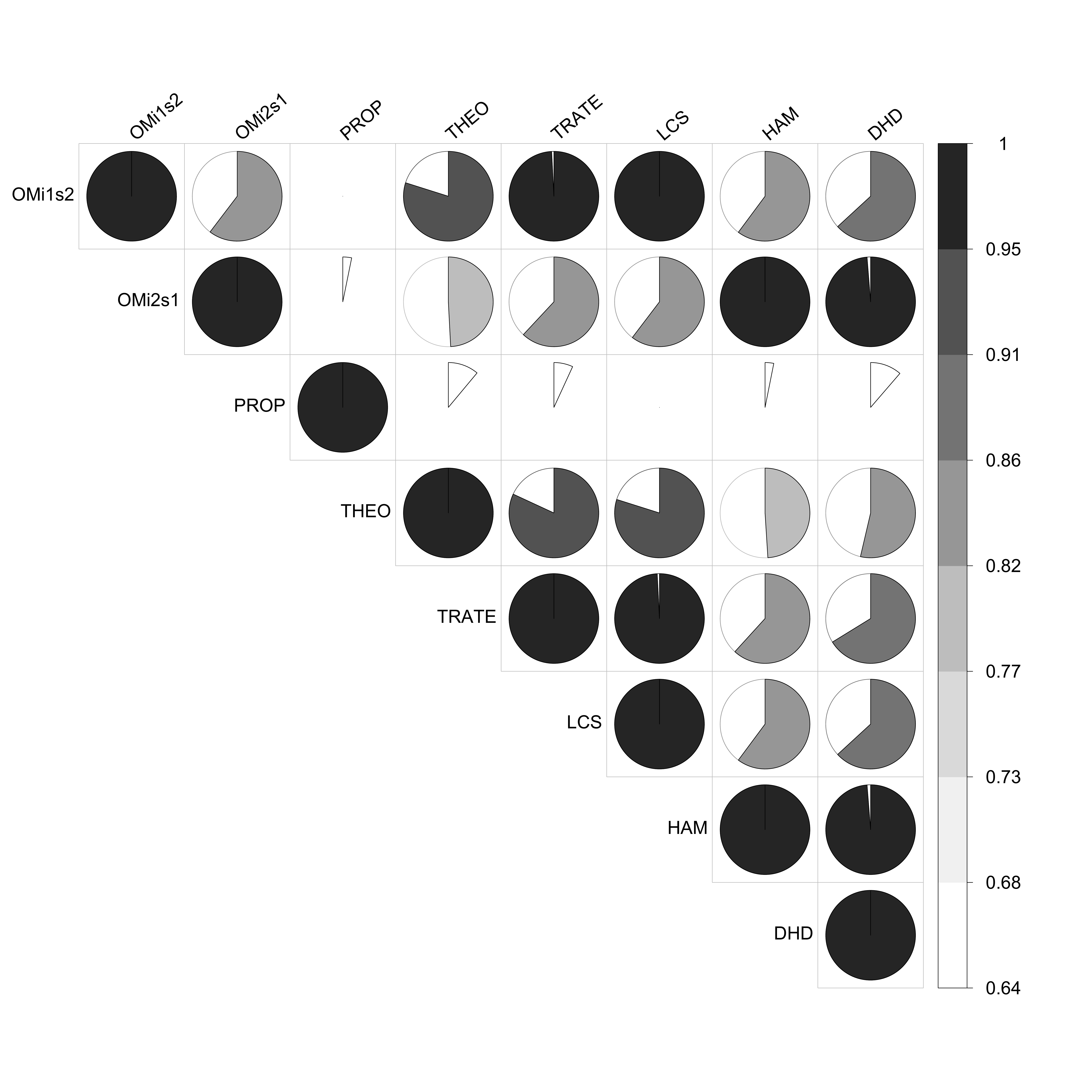
If you want to explore the code to produce this graph, here it is:

corrplot(corr.partner.child.n, 
         method =("pie"), 
         type = "upper", 
         tl.col = "black", 
         tl.srt = 40, 
         tl.cex = 2,
         cl.cex = 2,
         col=brewer.pal(n = 8, name = "Greys"),
         is.corr = FALSE)
dev.off()

Correlation for dissimilarity matrices

Preparatory work: computing the dissimilarity matrices to be compared

Correlation between the different dissimilarity matrices

Correlation between the different normalized dissimilarity matrices

Corrections

Reuse