Click here to get instructions…
- Please download and unzip the replication files for Chapter 3 ( Chapter03.zip).
- Read
readme.htmland run3-0_ChapterSetup.R. This will create3-0_ChapterSetup.RDatain the sub folderdata/R. This file contains the data required to produce the plots shown below. - You also have to add the function
legend_large_boxto your environment in order to render the tweaked version of the legend described below. You find this file in thesourcefolder of the unzipped Chapter 3 archive. - We also recommend to load the libraries listed in Chapter 3’s
LoadInstallPackages.R
# assuming you are working within .Rproj environment
library(here)

# install (if necessary) and load other required packages
source(here("source", "load_libraries.R"))

# load environment generated in "3-0_ChapterSetup.R"
load(here("data", "R", "3-0_ChapterSetup.RData"))
In chapter 3.3, we introduce alignment-based extensions of OM. The data come from a sub-sample of the German Family Panel - pairfam. For further information on the study and on how to access the full scientific use file see here.
Theory-based costs
We generate a substitution costs matrix to be used in the next step based on the following theory-based costs:
substitution=1 if one if different number of children but same partnership status
substitution=2 any substitution of different partnership statuses
theo <- matrix(
  c(0,1,2,2,2,2,2,2,2,
    1,0,2,2,2,2,2,2,2,
    2,2,0,1,2,2,2,2,2,
    2,2,1,0,2,2,2,2,2,
    2,2,2,2,0,1,2,2,2,
    2,2,2,2,1,0,2,2,2,
    2,2,2,2,2,2,0,1,1,
    2,2,2,2,2,2,1,0,1,
    2,2,2,2,2,2,1,1,0),
  nrow = 9,
  ncol = 9,
  byrow = TRUE,
  dimnames = list(longlab.partner.child,
                  shortlab.partner.child))
and display the resulting matrix:
theo S Sc LAT LATc COH COHc MAR MARc1 MARc2+
Single, no child 0 1 2 2 2 2 2 2 2
Single, child(ren) 1 0 2 2 2 2 2 2 2
LAT, no child 2 2 0 1 2 2 2 2 2
LAT, child(ren) 2 2 1 0 2 2 2 2 2
Cohabiting, no child 2 2 2 2 0 1 2 2 2
Cohabiting, child(ren) 2 2 2 2 1 0 2 2 2
Married, no child 2 2 2 2 2 2 0 1 1
Married, 1 child 2 2 2 2 2 2 1 0 1
Married, 2+ children 2 2 2 2 2 2 1 1 0We use this matrix to calculate pairwise dissimilarities:
om.theo<-seqdist(partner.child.year.seq, method = "OM", indel = 1,sm = theo)Let’s consider the first three sequences in the initial sample:
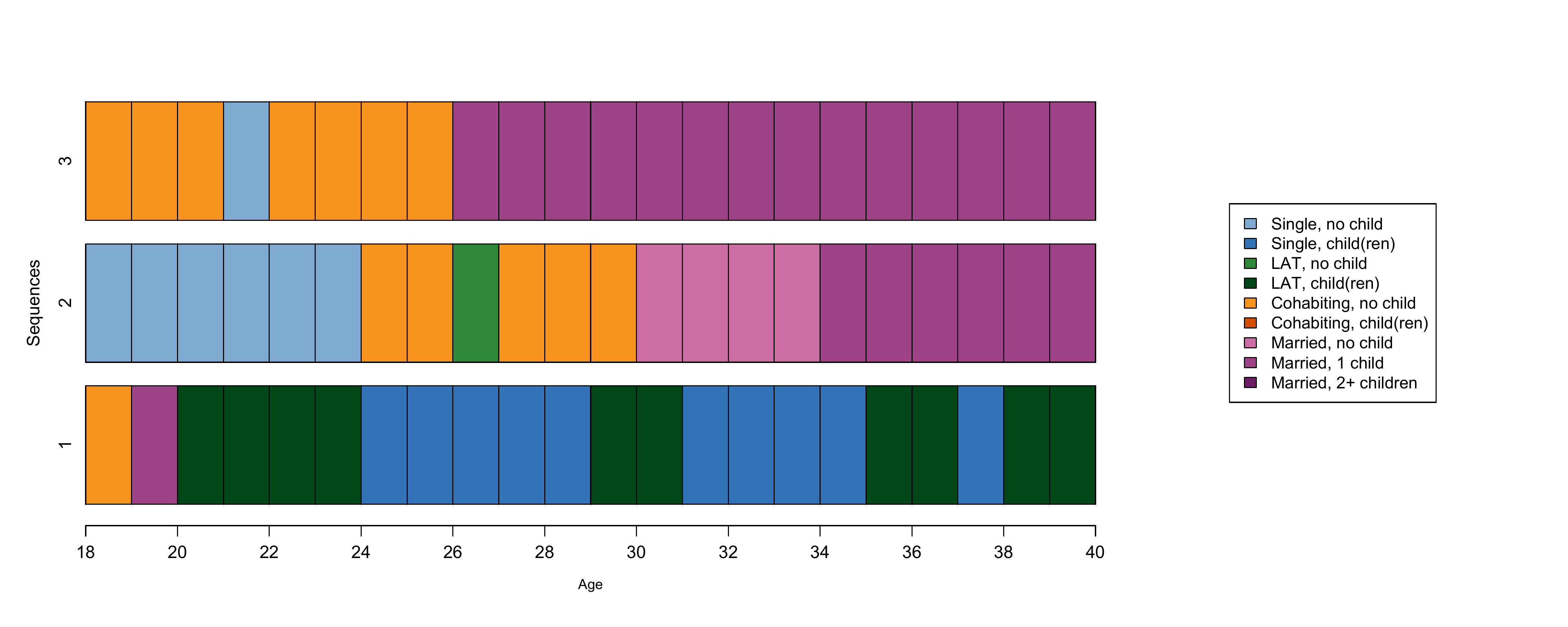
In the book, this corresponds to Figure 3.1: if you want to generate this figure in color as we do here, you can use the following code
layout.fig1 <- layout(matrix(seq(1:2), 1, 2, byrow = TRUE),
                      widths = c(.7, .3))
layout.show(layout.fig1)

par(mar = c(5, 4, 4, 0) + 0.1, las = 1,
    mgp=c(2,1,-.5))
seqiplot(partner.child.year.seq[1:3, ],
         ylab = "Sequences",
         with.legend = "FALSE",
         border = TRUE,
         axes = FALSE,
         cpal = colspace.partner.child,
         main = "",
         weighted=FALSE)
par(mgp=c(3,1,0.25))
axis(1, at=(seq(0,22, 2)), labels = seq(18,40, by = 2))
mtext(text = "Age", cex = .8,
      side = 1,#side 1 = bottom
      line = 2.5)

par(mar = c(5, 0, 4, 0) + 0.1)
seqlegend(partner.child.year.seq,
          cpal = colspace.partner.child,
          cex = .95, position = "center")

dev.off()
We can now inspect a selection of the dissimilarity matrix between the three sequences above:
om.theo[1:3, 1:3] 1 2 3
1 0 37 40
2 37 0 18
3 40 18 0Costs based on state properties
Generate two vectors with the following properties for each possible state:
 partner: 0=single, 1=couple
 child: 0=no, 1=yes
partner <- c(0, 0, 1, 1, 1, 1, 1,1,1)
child <- c(0,1,0,1,0,1,0,1,1)Create a data.frame with the vectors:
alphabetprop <- data.frame(partner = partner, child = child)Label the rows of the data.frame after the states’
names:
rownames(alphabetprop) <- alphabet(partner.child.year.seq)… and display the data.frame
alphabetprop partner child
S 0 0
Sc 0 1
LAT 1 0
LATc 1 1
COH 1 0
COHc 1 1
MAR 1 0
MARc1 1 1
MARc2+ 1 1Generate a substitution costs matrix based on the properties with “Gower” algorithm and print it
prop <- as.matrix(daisy(alphabetprop,
                        metric = "gower"))
prop
S Sc LAT LATc COH COHc MAR MARc1 MARc2+
S 0.0 0.5 0.5 1.0 0.5 1.0 0.5 1.0 1.0
Sc 0.5 0.0 1.0 0.5 1.0 0.5 1.0 0.5 0.5
LAT 0.5 1.0 0.0 0.5 0.0 0.5 0.0 0.5 0.5
LATc 1.0 0.5 0.5 0.0 0.5 0.0 0.5 0.0 0.0
COH 0.5 1.0 0.0 0.5 0.0 0.5 0.0 0.5 0.5
COHc 1.0 0.5 0.5 0.0 0.5 0.0 0.5 0.0 0.0
MAR 0.5 1.0 0.0 0.5 0.0 0.5 0.0 0.5 0.5
MARc1 1.0 0.5 0.5 0.0 0.5 0.0 0.5 0.0 0.0
MARc2+ 1.0 0.5 0.5 0.0 0.5 0.0 0.5 0.0 0.0Alternatively, this code can be used within the ?seqcost
command (where FEATURES corresponds to the properties)
prop2 <- seqcost(partner.child.year.seq,
method="FEATURES",
state.features = alphabetprop,
feature.weights = NULL)
prop2$indel
[1] 0.5
$sm
         S  Sc LAT LATc COH COHc MAR MARc1 MARc2+
S      0.0 0.5 0.5  1.0 0.5  1.0 0.5   1.0    1.0
Sc     0.5 0.0 1.0  0.5 1.0  0.5 1.0   0.5    0.5
LAT    0.5 1.0 0.0  0.5 0.0  0.5 0.0   0.5    0.5
LATc   1.0 0.5 0.5  0.0 0.5  0.0 0.5   0.0    0.0
COH    0.5 1.0 0.0  0.5 0.0  0.5 0.0   0.5    0.5
COHc   1.0 0.5 0.5  0.0 0.5  0.0 0.5   0.0    0.0
MAR    0.5 1.0 0.0  0.5 0.0  0.5 0.0   0.5    0.5
MARc1  1.0 0.5 0.5  0.0 0.5  0.0 0.5   0.0    0.0
MARc2+ 1.0 0.5 0.5 0.0 0.5 0.0 0.5 0.0 0.0We then use the matrix to calculate the pairwise dissimilarities, and display a selection of the dissimilarity matrix between sequences in the figure above (Fig. 3.1):
om.prop<-seqdist(partner.child.year.seq,
                 method = "OM",
                 indel = 1,
                 sm = prop)
om.prop[1:3, 1:3]
1 2 3
1 0.0 15.5 9.0
2 15.5 0.0 6.5
3 9.0 6.5 0.0Here an alternative code to use the matrix to calculate pairwise dissimilarities and display the dissimilarity matrix between the usual sequences (Fig. 3.1)
om.prop2<-seqdist(partner.child.year.seq,
                  method = "OM",
                  indel = 1,
                  sm = prop2$sm)
om.prop2[1:3, 1:3]
1 2 3
1 0.0 15.5 9.0
2 15.5 0.0 6.5
3 9.0 6.5 0.0Data driven-costs
For illustrative purpose, we use three example sequences (6 time-points, 3 states: A, B, C)
ch3.ex2 <- c("A-B-B-C-C-C", "A-B-B-B-B-B", "B-C-C-C-B-B")

ch3.ex2.seq <- seqdef(ch3.ex2)
The command ?seqcost generates substitution costs, in
this case based on transition rates. The command returns also the value
of indel.
trate1<-seqcost(ch3.ex2.seq, method="TRATE")We can display the substitution costs matrix based on transition rates
trate1$indel
[1] 1
$sm
  A    B    C
A 0 1.00 2.00
B 1 0.00 1.55
C 2 1.55 0.00As an alternative code, ?seqsubm generates substitution
costs (here based on transition rates as above), but does not return
indel
trate2 <- seqsubm(ch3.ex2.seq, method="TRATE")We can display the substitution costs matrix based on transition rates
trate2 A B C
A 0 1.00 2.00
B 1 0.00 1.55
C 2 1.55 0.00We now want to extract the transition rates between states for the three example sequences:
tr.rates<-seqtrate(ch3.ex2.seq, sel.states = NULL,
                   time.varying = FALSE,
                   weighted = TRUE,
                   lag = 1,
                   with.missing = FALSE,
                   count = FALSE)
…and use the ?seqalign command to get a summary of the
optimal number and costs of OM operations with data-driven (transition
rates) substitution costs:
al1.OM.dd <- seqalign(ch3.ex2.seq, 1:2,
                      indel=1,
                      sm=trate2)

print(al1.OM.dd)
1 2 3 4 5 6
Seq 1 A B B C C C
Operations E E E S S S
Costs 0.00 0.00 0.00 1.55 1.55 1.55
Seq 2 A B B B B B
OM distance between sequences: 4.65 al2.OM.dd <- seqalign(ch3.ex2.seq, c
(1,3),
indel=1,
sm=trate2)
print(al2.OM.dd) 1 2 3 4 5 6 7 8
Seq 1 A B B C C C - -
Operations D D E E E E I I
Costs 1 1 0 0 0 0 1 1
Seq 2 - - B C C C B B
OM distance between sequences: 4 al3.OM.dd <- seqalign(ch3.ex2.seq,
2:3,
indel=1,
sm=trate2)
print(al3.OM.dd) 1 2 3 4 5 6 7
Seq 1 A B - B B B B
Operations D E I S S E E
Costs 1.00 0.00 1.00 1.55 1.55 0.00 0.00
Seq 2 - B C C C B B
OM distance between sequences: 5.1 Dynamic Hamming distance
We proceed by using the three example sequences and compute the
dissimilarity matrix using the following costs: indel=1,
sm=dynamic Hamming distance (DHD)
dhd.diss<-seqdist(ch3.ex2.seq,
                  method="DHD")
…and display the resulting DHD-based dissimilarity matrix:
dhd.diss [1] [2] [3]
[1] 0.0 10.5 16.0
[2] 10.5 0.0 11.5
[3] 16.0 11.5 0.0